Planetary

Radiative transfer analysis

There are numerous available radiative transfer models, yet these packages typically require complex installation and compilation procedures for them to operate, and they are particularly restrictive in operational scope (e.g., planet, type of atmosphere/surface) and wavelength (e.g., spectral database, file formats). For instance at the internet encyclopedia (Wikipedia), there is an entry for "Atmospheric radiative transfer codes", listing dozens of packages and their capabilities (wavelength range, geometry, scattering, polarization, accessibility/licensing, etc.). There have been several attempts to quantify the differences between different packages (e.g., Alvarado et al. 2013), and a commercial internet facility (www.spectralcalc.com) implements a small subset relevant to Earth/Mars science.
 
With this online tool, we pursue to provide to the community an accurate and comprehensive (UV/Vis/IR/mm) planetary tool, allowing to synthesize realistic spectra for a broad range of objects (rocky planets, gas giants, icy bodies, TNOs, comets, exoplanets, etc.), and assisting with the planning and execution of current and future NASA missions. This is achieved by integrating two core radiative-transfer models: the accurate and versatile PUMAS atmospheric/scattering model, and the cometary emission model (CEM).
 

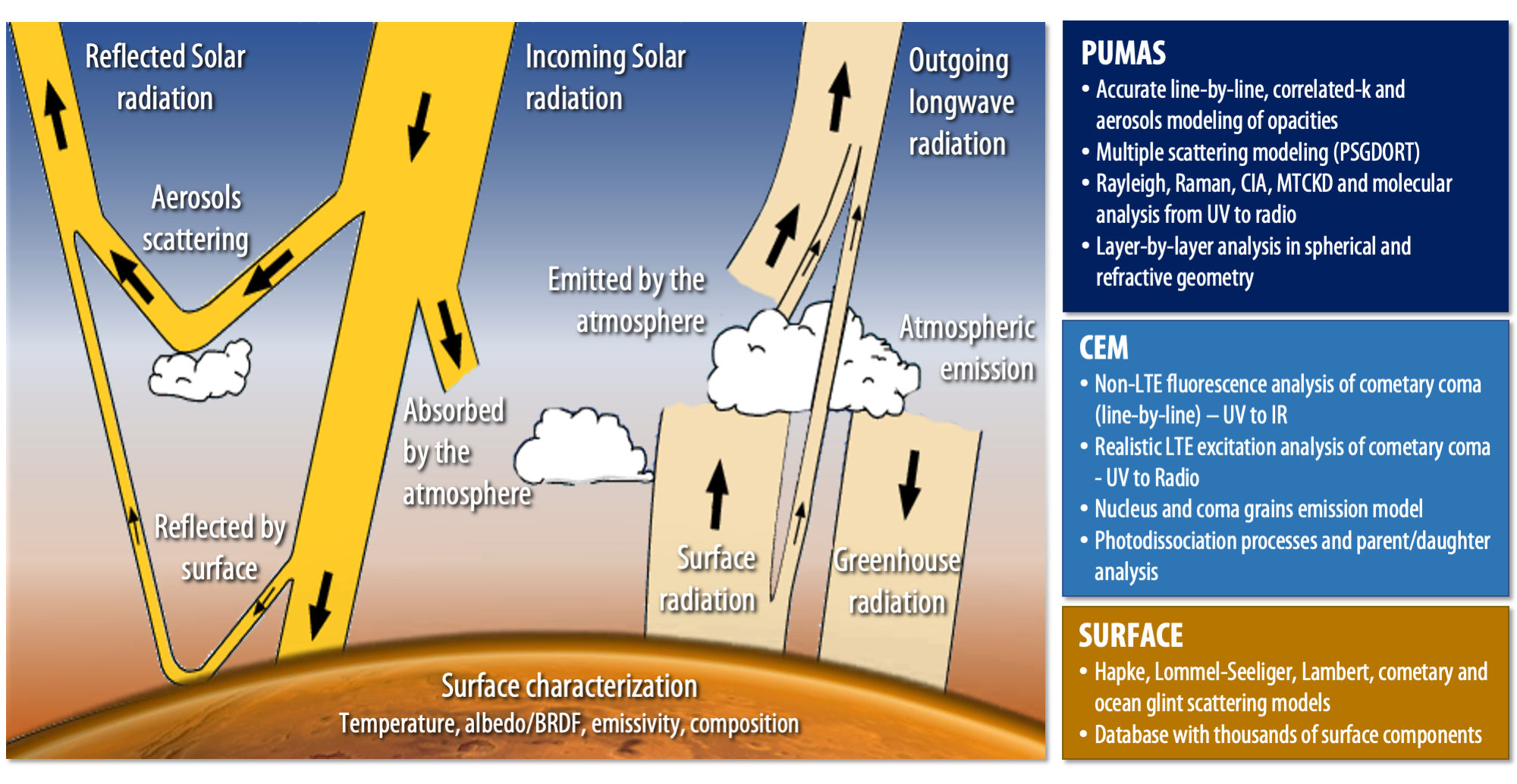Components of the PSG radiative transfer: the diagram shows the different components considered by the radiative transfer modules. By performing a layer-by-layer analysis, PUMAS intrinsically integrates and calculates the different flux contributions across the wavelength grid. For comets, the molecular calculation is performed separately by CEM from the surface fluxes, and later added to compute integrated fluxes.

Atmospheric radiative transfer models

In order to compute atmospheric transmittances and radiances, the molecular modules ingest the parameters defined in the "atmosphere" section and compute observable fluxes:
 

Linelist	Capabilities	Reference
PUMAS Planetary and Universal Model of Atmospheric Scattering	PUMAS integrates the latest radiative-transfer methods and spectroscopic parameterizations, in order to compute high resolution spectra via line-by-line calculations, and utilizes the efficient correlated-k method at moderate resolutions. The scattering analysis is based on a Martian scattering model (Smith et al. 2009), while the line-by-line calculations have been validated and benchmarked with the accurate GENLN2 model (Edwards 1992).	Villanueva, G. L. et al., Science, Volume 348, Issue 6231, pp. 218-221 (2015). Smith, M. D. et al., JGR, Vol. 114, E00D03, (2009). Edwards, D. P., "GENLN2: A general line-by-line atmospheric transmittance and radiance model, Version 3.0 description and users guide", NCAR/TN-367-STR, National Center for Atmospheric Research, Boulder, Co. (1992).
CEM Cometary Emission Model	CEM incorporates excitation processes via non-LTE line-by-line fluorescence model at short wavelengths (employing GSFC databases), and ingests several spectral databases to compute line-by-line LTE fluxes. It operates with expanding coma atmospheres and temperatures lower than 300K, and accurately computes photodissociation processes for parent and daugther species released in the coma.	Villanueva, G. L. et al., The molecular composition of Comet C/2007 W1 (Boattini): Evidence of a peculiar outgassing and a rich chemistry. Icarus, Volume 216, Issue 1, p. 227-240 (2011) Villanueva, G. L., The High Resolution Spectrometer for SOFIA-GREAT: Instrumentation, Atmospheric Modeling and Observations. PhD Thesis, Albert-Ludwigs-Universitaet zu Freiburg, ISBN 3-936586-34-9, Copernicus GmbH Verlag (2004)
MASS Mass Advanced Spectrometry Simulator	MASS interprets complex mass fragmentation moleculer patterns and computes high-resolution mass spectra of orbiters, landers and laboratory instrumentation. The fragmentation patterns are pre-computed by permutation theory for all possible isotopologues of the molecular fragments. MASS computes local densities in hydrostatic atmospheres and in cometary coma by employing accurate atmospheric evolution and photodissociation calculations.	Villanueva, G. L. et al., MASS: Mass Advanced Spectrometry Simulator, see chapter 7

 

Sampling of the planetary disk

General Circulation Model (GCM) sampling (heterogeneous atmospheric/surface properties and geometries)

Realistic modeling of full disk and transit planetary fluxes requires to capture the heterogeneous properties of the atmosphere and the surface across the observable disk and the terminator. PSG allows to ingest General Circulation Model (GCM) 3D data of temperature, pressure and abundance profiles, together with surface properties, such as albedo. The user can upload atmospheric data from any GCM, after converting the 3D fields (typically in netCDF format) into a PSG GCM binary file. The 3D and temporal atmospheric data are then aggregated and mapped into a 2D projected observationally grid that is fed to the radiative transfer modules. PSG currently provides templates and conversion scripts for several GCM models, including the Rocke3D terrestrial model, the Laboratoire de Météorologie Dynamique (LMD) model, the Community Atmosphere Model (CAM) model, and the Unified Model (UM). In order to ingest GCM 3D data, these are the steps required:
 
1) Run the GCM model in your personal machine, and store the resulting 3D fields and parameters into a GCM formatted file (typically a netCDF file).
 
2) By employing a script (see scripts in GitHub) convert the GCM netCDF file into a PSG GCM binary file. Several example conversion scripts are available at the GlobES application site, permitting to convert netCDF ouput files from Rocke3D, LMD and CAM. This script should be run at the user's local machine.
 
3) In the GlobES site, upload the PSG GCM file by clicking on "Load GCM data". If the upload process was successful, the site should display graphically the GCM outputs for the different variables.
 
4) Select the observing geometry (e.g., transit, direct imaging) directly on the GlobES site, or at the "Target and Geometry" section of PSG, and verify and update the molecules and aerosols to include in the simulation by visiting the "Atmosphere and Surface" section of PSG.
 
5) In the GlobES site, click on "Generate 3D spectra". For each position on the planet, the algorithm will update the atmospheric profiles, surface properties and geometry parameters and will run the radiative transfer. These results will be integrated employing the appropiate weights. Results will be displayed in the "Home" site of PSG.
 
To run the GlobES module in script mode via the API, please check the python scripts available in GitHub.
 
Binning: to speed up the calculations one can horizontally bin/aggregate GCM data to have less PSG radiative-transfer calculations. Higher binning means more aggregation and less PSG radiative-transfer calculations. High "binning" numbers (above 50) should only be used when testing. A "binning" factor of 3 is typically recommended, leading to 3 x 3 (lat x lon = 9) binning, and a speed up of 9 times while sacrificing a little accuracy.
 

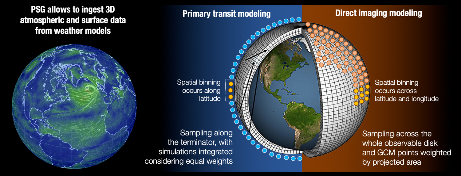Simulation of realistic spectra employing 3D GCM data: ingestion of 3D atmospheric data is possible in PSG, and this allows to accurately capture the heterogenity of the atmospheric and the surface across the observable disk and terminator. For transit observations, the GlobES algorithm performs radiative transfer simulations across the terminator, and integrates the different spectra employing equal weights. For direct imaging and secondary eclipse simulations, the algorithm performs radiative transfer simulations across the whole observable disk, and the individual spectra are integrated considering the projected area of each bin.

 

Radiative transfer sampling (homogeneous atmospheric/surface properties, heterogeneous geometries)

Simulations that encompass the whole observable disk would require sub-sampling in order to properly capture the diversity in incidence and emission angles. Specifically, when the FOV is much smaller than the object disk (e.g., nadir, limb, occultation and looking-up observations), a single set of geometry parameters is typically sufficient when performing the radiative transfer calculation. The issue is when the FOV samples a broad range of illuminations and surface properties (e.g., the FOV is comparable and/or bigger than the object disk); in this case, one would need to compute radiative transfer simulations over different geometries, which would be then integrated to produce a single total planetary flux. By default, PSG currently defines one set of geometry parameters and one radiative-transfer calculation per simulation, yet we integrated into PSG an algorithm that allows to sub-sample the observable disk into sub-sections of similar incidence / emission angles.
 
The algorithm takes as input N, or the disk sub-sampling parameter (entered in the target section), which defines the number of angle bins for the incidence and emission angles. Since these angles range from 0 to 90, a N=5 would lead to a sub-division with bins of 18° and leading to 22 distinct radiative-transfer regions as described in the figure below. The computational requirement scales quadractic with N, so a conscious choice has to be made between accuracy and performance. The default is N=1, leading to typical errors less than 5% in flux, while N=3 reaches typical errors lower than 1%, and N=10 reaches flux accuracy better than 0.1%.
 

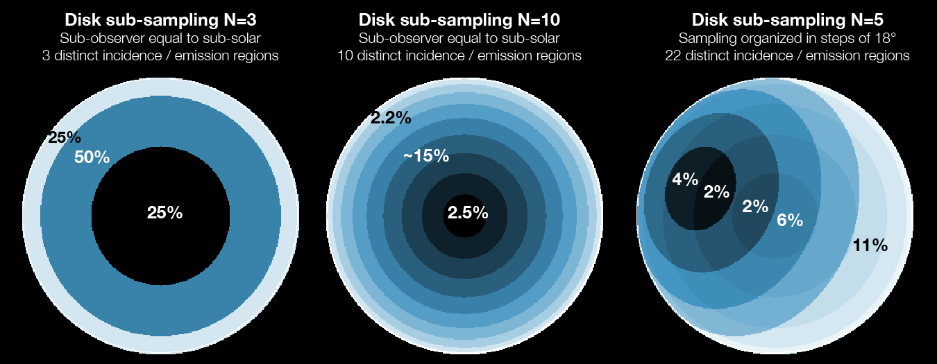Disk sampling methodology: when the beam samples a broad range of incidence and emission angles, PSG allows to divide the observable disk into sub-sections of similar incidence / emission angles. The sampling parameter (N, disk sub-sampling) defines the number of angle bins for the incidence and emission angles. Typically, N=3 reaches errors lower than 1%, and N=10 reaches a flux accuracy better than 0.1%.

 

Atmospheres in disequilibrium (non-LTE)

In situations when collissions are infrequent enough to equilibrate the radiative populations of the molecules, an atmosphere is considered to be in non local thermodynamical equilibrium (non-LTE). When this occurs, the classical equations of Boltzmann distribution for populations and Planck's function for the source radiation terms are no longer valid. This primarily occurs in the tenous regions of the atmosphere, where collissions are infrequent and solar radiation is strong and unattenuated, leading to strong emissions as the molecules cascade back to their ground state. The radiative equilibrium equation for a two-level system can be written as:

n_u/n_l = (g_u/g_l) exp(-kcv/KT) [ (1 + ρB_lu/C_lu) / (1 + A_ul/C_ul) ]

where n are the populations of the upper (u) and lower (l) levels, g the statistical weights, T the local kinetic temperature, C_lu and C_ul the collisional excitation and relaxation rates respectively, B_lu and A_ul being Einstein coefficients for photo-absorption and spontaneuous emission, and ρ the impinging excitation flux. The Einstein coefficients are radiative properties of the levels in question, while the collision rates are dependent on the local temperature (α √T) and density. At high pressures, collisions dominate the radiative processes (C ≫ A_ul or C ≫ B_lu), and the relative populations of the levels can be simply described by Maxwell–Boltzmann statistics (LTE) dependent on the local kinetic temperature. In regions with strong external radiative fields (ρ), and more infrequent collisions (C ≪ A_ul or C ≪ B_lu), the radiative parameters start to define the energy balance of the molecule and its emitting spectrum (non-LTE).
 
As nicely summarized by Appleby (1990), non-LTE starts to become relevant for methane in the atmosphere of giant planets (e.g., Jupiter, Saturn, Uranus, Neptune) in the mesosphere at pressures below 0.1 mbar. In CO₂ rich atmospheres (e.g., Mars, Venus), the efficient collisional rates for this molecule, keeps LTE up to much lower densities (> 1 ubar, Lopez-Puertas & López-Valverde 1995). In the atmospheres of hot-giants, stronger radiation fields will bring this limit deeper into the atmosphere, while higher kinetic temperatures will keep LTE further up in the atmosphere. Chemical reactions also lead molecules into highly excited non-equilibrium states, from which diagnostic photons are released, as it is the case for the dayglow O₂(¹Δ) emission tracking the photodestruction of O₃ in terrestrial atmospheres (Novak et al. 2002).
 
Implementation of non-LTE in PSG: the radiative transfer module of PSG, PUMAS, allows to ingest non-equilibrated populations for the energy levels, and it will use these to compute the opacity and source functions for every ro-vibrational level at each layer (Kutepov et al. 1998). Specifically, PSG permits to model the most common case of non-LTE, in which the vibrational levels are assumed to be in disequilibrium while the rotational populations are assumed to be equilibrated. For that purpose, the user must provide vertical profiles of vibrational temperatures [K] (computed relative to the ground-state) for every isotopologue and vibrational band, in the form of "Tvib[MOL:ISO:IDvib]" (MOL:HITRAN molecular ID, ISO:Isotopologue ID, IDVib: vibrational band ID as defined for the isotopologue [see vibrational bands in the linelist help]). For instance "Tvib[6:1:7]" would correspond to the v3=1 level of the main isotope of CH₄.
 

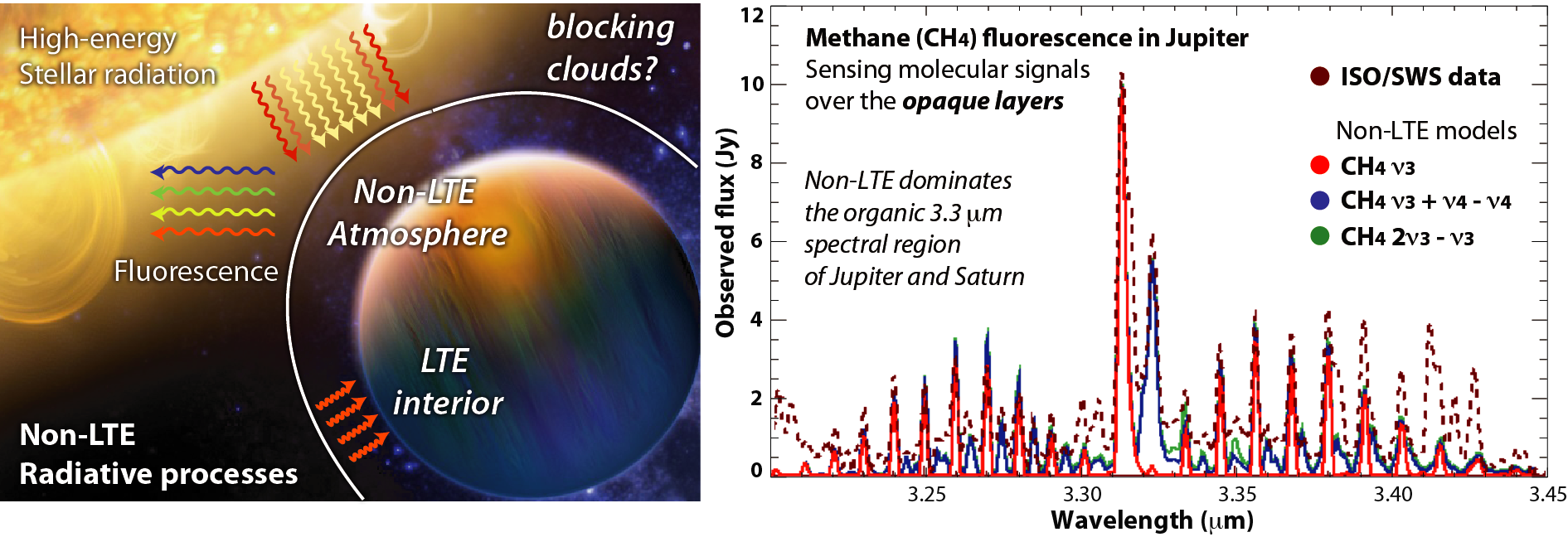Modeling of non-LTE radiation: As the atmospheres are bombarded by high-energy photons from their partner stars, the upper-layers emit efficiently via non-LTE processes. This disequilibrium has been observed across many planets in our solar system (shown is the detection of non-LTE methane in Jupiter; Encrenaz et al. 1996; Drossart et al. 1999), and is certainly active in many exoplanets’ atmospheres.

 

Retrieval methods

PSG allows to compare user-provided data to synthetically generated spectra, and to perform physical retrievals of the parameters included in the model employing the optimal estimation method (Rodgers 2000). The retrieval module also implements an additional regularization parameter that improves the retrieval accuracy and convergence speed of the inverse scheme. The optimal estimator that PSG uses to get an estimate of the parameters from observations is obtained by considering a linear Gauss–Newton iterative scheme. The formal retrieval equation implemented follows this scheme:
 

x (γS_a^-1  +  K^TS_y^-1K)  =  y (K^TS_y^-1)

The scheme is based on the a-priori information available for the variability of the input quantities and the knowledge of the measurement uncertainty; if no error is provided, PSG will assume a 5% uncertainty. The minimum/maximum limits entered in the form for each parameter as assumed to be 5-sigma, and therefore the "variance" of each parameter is defined as (maximum-minimum)/10. Both covariance matrices, data and parameters, are assumed to be diagonal and filled with the squares of the data and parameter variances, respectively. The Jacobians are computed with forward steps of 0.1% of the maximum value.
 
The parameter γ is the extra regularization parameter, and acts as a tradeoff between the a-priori values given to the parameters to be retrieved (x-space) and the observations (y-space). Large values of γ will constrain the retrieval scheme more to the a-priori parameter values, hence a large γ might be recommended in case of reliable a-priori knowledge of retrieval parameters. As γ approaches 0, the solution scheme tends to a constrained least-square. For γ = 1, the Rodgers’ classical scheme is run.
 
Together with the optimal estimate for the parameters, the retrieval module implemented in PSG computes a series of a-posteriori quantities. The uncertainties of the parameters are computed from the a-posteriori covariance matrix, which is directly derived from the Rodgers’ formalism. In addition, the averaging kernels matrix (AK) is computed for each of the retrieved parameters. AKs provide information about the information content of the data with respect to the retrieved parameters. The diagonal of the AK matrix contains values between 0 and 1, which indicate the sensitivity of the retrieval to each parameter. Low values could be indicative of intrinsic poor sensitivity of the data themselves to the retrieval parameters, or could be due to very stringent constraints imposed to the variability of the parameters to be retrieved. In general, the contribution functions matrix and the AKs are presented to highlight the properties of the retrieved parameters, and their significance. AKs can also be provided prior to the retrieval, to allow the user to evaluate the information content of the spectrum, and tune the input parameters. The retrieval provides also an accurate a-posteriori estimation of the measurement uncertainty.
 
Beyond fitting the data to the spectroscopic model, PSG can also correct for a broad range of instrumental issues typically affecting data (see the figure below). By employing pre-computed telluric spectra, PSG can also fit the water and column parameters affecting ground-based data. For fitting these instrumental effects, PSG employs the Levenberg–Marquardt algorithm, also known as the damped least-squares method, in solving the non-linear least squares problem. This method interpolates between the Gauss–Newton algorithm and the method of gradient descent, with the Levenberg–Marquardt method being more robust, meaning that it finds a solution even if the initial conditions are far from the final solution. The Levenberg-Marquardt algorithm is based on the MPFIT program (Craig Markwardt), which draws from the robust package called MINPACK-1 (Garbow, Hillstrom and More).
 

Optimal Estimation Method (OEM) C/C++ package Developed by Liuzzi and Villanueva, Sep/2018 Based on methodologies described in Rodgers 2000 and therein.	Download
Levenberg-Marquardt (LM) minimization C/C++ package Developed by Craig Markwardt, June/2016 Based on the MINPACK-1 (Garbow, Hillstrom and More).	Download

 
The input file should be formatted as a text file with two or three columns. The first column should indicate the frequency/wavelength of each pixel, while the second column should describe the measured flux. A third column (optional) should indicate the 1-sigma uncertainty in flux, and if no error is provided, PSG will assume a 5% uncertainty. See below a list of example configuration files (that also include the data):

• Comet IR retrieval: retrieval of production rates and rotational temperatures in comet C/2007 W1 (Boattini) from high-resolution Keck/NIRSPEC data acquired on July/9/2008 (Villanueva et al. 2011, Icarus 216, 227-240).
• Mars retrieval: retrieval of deuterated water from high-resolution Keck/NIRSPEC data acquired in January/2014. This is a relatively complex and expensive retrieval, in which several instrumental issues are removed simultaneously (Villanueva et al. 2015, Science 348-6231).
• Comet radio retrieval: retrieval of cometary methanol production rate and its rotational temperature from high-resolution data of comet C/2002 T7 (LINEAR) acquired with the Heinrich Hertz Submillimeter Telescope (Villanueva et al. 2005, AAS/DPS meeting).
• Earth retrieval: retrieval of methane and carbon dioxide in Earth's atmosphere via laser heterodyne radiometry (LHR). This is part of a ground-based network of stations located across the planet (Wilson et al. 2017).

 

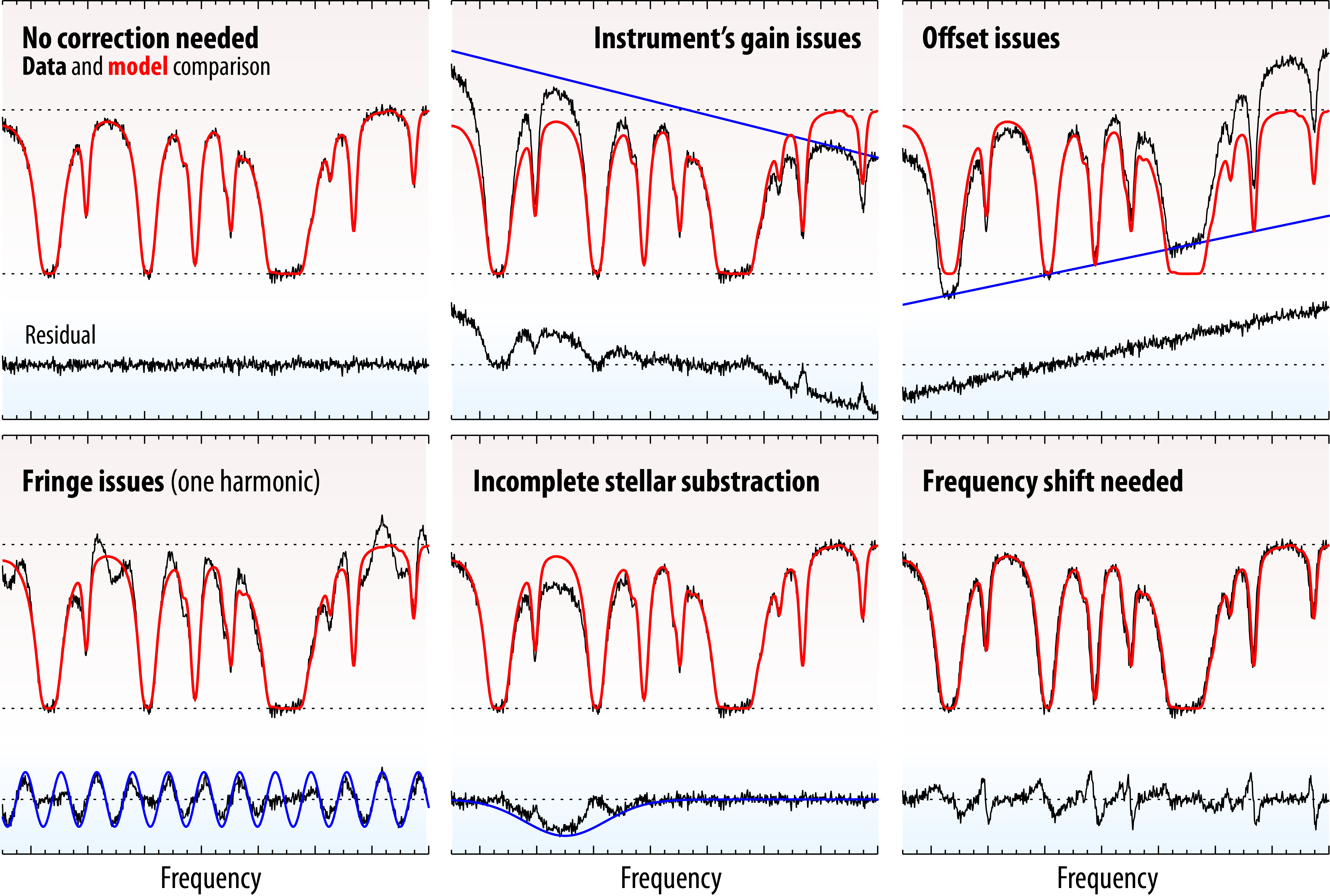Data corrections: beyond performing the retrieval of planetary parameters, PSG can also correct for several typical issues affecting spectroscopic data. The different panels show how these issues could affect the data, and their impact on the residuals. The methods employed to remove these instrumental effects are described in Villanueva et al. 2013 (Icarus 223, 11–27).

Instrument parameters

In this section, the user defines the desired characteristics of the synthetic spectra (wavelength range, resolution, desired radiance flux, noise performance, etc.). When observing with ground-based observatories, PSG allows to affect the synthetic spectra by telluric absorption. The tool has access to a database of telluric transmittances pre-computed for 5 altitudes and 4 columns of water for each case (20 cases in total). The tool can also perform noise (and signal-to-noise ratio) calculation by providing details about the detector and the telescope performance.
 
PSG allows to define several type of telescope/instrument modes, while in all cases, the integration of the fluxes is done over bounded and finite field-of-views and spectral ranges, with no convolutions applied to the fields.

• Single telescope: this mode is the classical observatory / instrument optical setup, in which the etendue is defined by the effective collecting area of the main mirror A_Tele and its corresponding solid angle Ω.
• Interferometer: this mode is characterized by an etendue that is proportional to the number of antennas (e.g., ALMA), in which A_Tele = n_Tele⋅π⋅[D_Tele/2]².
• Coronagraph: In a coronagraph model, the stellar fluxes are attenuated by the contrast, while the the planetary and background signatures are attenuated by the coronagraph transfer function, which is dependent on the working angle (L/D). The user can provide detailed transfer functions for the coronagraph, while PSG has curves for several observatories. If no coronagraph function is provided, PSG assumes that the throughput is minimum (contrast) within half the inner-working-angle (IWA), it reaches 0.5 at the IWA, and reaches 1.0 at 1.5 times the IWA. Relevant to this mode is also the "Exozodi" level, which indicates the level of zodiacal dust in the exoplanetary system w.r.t to Earth's zodiacal fluxes (see below).
• AOTF+grating: this mode characterizes telescope/instruments in which an Acousto-Optical-Tunable-Filter (AOTF) is located between the entrance optics and the spectroscopic grating (e.g., ExoMars/TGO). The AOTF can be described with 6-parameters (only the center is required): center [cm^-1], width [cm^-1], sidelobes factor, base, gauss width [cm^-1], factor. The grating is described with 2 parameters: center [cm^-1, required] and width [cm^-1].
• LIDAR system: in this mode, the "laser" source is injected in the FOV as an additional radiation flux, with the beam [FWHM] describing the laser divergence of the source, and D_Tele the diameter of the receiver. Two parameters describe the laser intensity, its peak power [W] and the duty cycle [%] (ON/ON+OFF). The integration time is considered to be for the complete spectral scan, so an integration time of 1 sec for 100 spectral points, would correspond to an integration time of 10 ms per spectral point. The standard case assumes that the receiver is colocated with the laser-source for nadir/observatory geometries (with the surface behaving as a Lambertian), while for limb geometries, PSG assumes that the receiver is located at the other side of the occultation. When entering a second value in the duty-cycle field, one defines that the receiver/source are also colocated for limb geometries, with this additional value defining the reflectivity of the reflector at the other side of the occultation.

We have compiled a database of instrument models for a diverse range of telescope/instrument combinations, assisting the user when defining the basic parameters of the instrument. Additional instrument models are being developed.
 

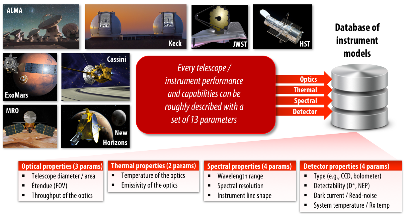Instrument model: We have identified 13 key parametes that are sufficient to describe the overall capabilities and performance of a particular telescope/instrument combination, and we are now in the process of compiling a database of instrument models, that will assist the user when defining the basic parameters of the instrument.

Echelle simulator

We have developed an echelle simulator for iSHELL (Immersion Grating Echelle Spectrograph) at the NASA Infrared Telescope Facility (IRTF). It employs a set of ab-initio grating equations and simplified parameters that are accurate enough to describe the overall behavior of the cross-dispersors and the gratings.

 

Radiance and wavelength units

PSG allows to compute synthetic fluxes in a broad range of possible units. The constants used for the conversion are: λ is the wavelength in microns (μm), c is the speed of light (299792458 m/s), ASR is arcseconds² per steradian (4.2545166E+10), h is Planck's constant (6.6260693E-34 W s²), k is Boltzmann's constant (1.380658E-23 J/K), A_Tele is the total collecting area of the observatory (m², n_Tele⋅π⋅[D_Tele/2]²), Ω is the field-of-view of the observations (steradian).
 

Quantity	Units	Formula	Keyword
Spectral radiance	W / sr / m2 / μm	L - This is the intrinsic unit of the modules	Wsrm2um
	W / sr / m2 / cm-1	L' = L ⋅ λ2 / 1E4	Wsrm2cm
	W / sr / m2 / Hz	L' = L ⋅ λ2 / (1E6 ⋅ c)	Wsrm2Hz
	Jy / arcsec2	L' = L ⋅ λ2 / (ASR ⋅ c) ⋅ 1E20	Jyarc
	K (brightness)	L' = PT / ln(1 + (PF/L)) PT = 1E6 ⋅ hc/kλ PF = 2E24 ⋅ hc2 / λ5	K
	K (Rayleigh-Jeans)	L' = L ⋅ 1E-18 ⋅ λ4 / 2kc	KRJ
Radiance	W / sr / m2	L' = L ⋅ dλ	Wsrm2
	Rayleigh	L' = L ⋅ dλ ⋅ 4π ⋅ λ ⋅ 1E-16 / hc	Ra
Spectral intensity	W / sr / μm	I = L ⋅ ATele	Wsrum
	W / sr / cm-1	I = L ⋅ ATele ⋅ λ2 / 1E4	Wsrcm
Radiant intensity	W / sr	I = L ⋅ ATele ⋅ dλ	Wsr
Spectral flux	W / μm	F = L ⋅ ATele ⋅ Ω	Wum
	W / cm-1	F = L ⋅ ATele ⋅ λ2 / 1E4 ⋅ Ω	Wcm
Radiant flux	W	F = L ⋅ ATele ⋅ Ω ⋅ dλ	W
	Photons / s	F = L ⋅ ATele ⋅ Ω ⋅ dλ ⋅ λ ⋅ 1E-6 / hc	ph
Integrated flux	Photons	F = L ⋅ texp ⋅ nexp ⋅ ATele ⋅ Ω ⋅ dλ ⋅ λ ⋅ 1E-6 / hc	pt
	Photons measured	F = L ⋅ neff ⋅ texp ⋅ nexp ⋅ ATele ⋅ Ω ⋅ dλ ⋅ λ ⋅ 1E-6 / hc	pm
Irradiance	W / m2	E = L ⋅ dλ ⋅ Ω	Wm2
	erg/s / cm2	E = L ⋅ dλ ⋅ Ω ⋅ 1E3	erg
Spectral irradiance	W / m2 / μm	E = L ⋅ Ω	Wm2um
	W / m2 / cm-1	E = L ⋅ Ω ⋅ λ2 / 1E4 ⋅	Wm2cm
	Jy	E = L ⋅ Ω ⋅ λ2 / c ⋅ 1E20	Jy
	mJy	E = L ⋅ Ω ⋅ λ2 / c ⋅ 1E23	mJy
Relative	Contrast	T = L / Lstellar	rel
	Transmittance (I/F)	T = L / Lcont	rif
	Magnitude	m = -2.5 ⋅ log(L ⋅ Ω / LVega)	V

 

Online unit conversion tool

Input	Output
Radiation value: From radiation unit: Photons/s (radiant flux) W (radiant flux) W/um (spectral flux) W/cm-1 (spectral flux) W/sr (radiant intensity) W/sr/um (spectral intensity) W/sr/cm-1 (spectral intensity) W/sr/m2 (radiance) W/sr/m2/um (spectral radiance) W/sr/m2/cm-1 (spectral radiance) W/sr/m2/Hz (spectral radiance) Jy/arcsec2 (spectral radiance) K (spectral radiance, brightness T) K Rayleigh-Jeans (spectral radiance, radio brightness T) W/m2 (irradiance) erg/s/cm2 (irradiance) W/m2/um (spectral irradiance) W/m2/cm-1 (spectral irradiance) Jy (spectral irradiance) m (spectral irradiance, apparent magnitude) To radiation unit: Photons/s (radiant flux) W (radiant flux) W/um (spectral flux) W/cm-1 (spectral flux) W/sr (radiant intensity) W/sr/um (spectral intensity) W/sr/cm-1 (spectral intensity) W/sr/m2 (radiance) W/sr/m2/um (spectral radiance) W/sr/m2/cm-1 (spectral radiance) W/sr/m2/Hz (spectral radiance) Jy/arcsec2 (spectral radiance) K (spectral radiance, brightness T) K Rayleigh-Jeans (spectral radiance, radio brightness T) W/m2 (irradiance) erg/s/cm2 (irradiance) W/m2/um (spectral irradiance) W/m2/cm-1 (spectral irradiance) Jy (spectral irradiance) m (spectral irradiance, apparent magnitude)   Frequency/wavelength: um nm mm Angstrom cm-1 MHz GHz kHz Resolving power: Field-of-view: arcsec arcmin degree steradian Telescope diameter [m, effective]:	1.4498685715765913e-11
Frequency / wavelength value: From unit: um nm mm Angstrom cm-1 MHz GHz kHz       To unit: um nm mm Angstrom cm-1 MHz GHz kHz	1.0

Telluric absorption

When observing with ground-based observatories, PSG allows to affect the synthetic spectra (or simply show) by telluric absorption. The tool has access to a database of telluric transmittances pre-computed for 5 altitudes and 4 columns of water for each case (20 cases in total). The altitudes include that of Mauna-Kea/Hawaii (4200 m), Paranal/Chile (2600 m), SOFIA (14,000 m) and balloon observatories (35,000 m), while the water vapor column was established by scaling the tropical water profile by a factor of 0.1, 0.3 and 0.7 and 1.
 
Opacities at 225 GHz, a typical metric to quantify water at radio wavelengths, can be estimated from the reported water column as τ225_PSG = 0.0642 x PWV, where PWV is the ammount of water in precipitable millimeters.
 

Noise simulator

PSG currently includes a noise calculator for quantum and thermal detectors, with the primary goal of providing users with quick look simulations for planning observations, and to assist with the development of new instrument/telescope concepts. The user can provide a constant value across all wavelengths (RMS), or a constant value with background noise (BKG), or can choose from several detector noise simulators.
 
At short wavelengths (e.g., optical or near IR), the background photon counts follow a Poisson distribution, and the fluctuations are given by √N where N is the mean number of photons received (see review in Zmuidzinas et al. 2003). This Poisson distribution holds only in the case that the mean photon mode occupation number is small, n<<1. For a thermal background, the occupation number is given by the Bose-Einstein formula, n_th(v,T) = [exp(hv/kT)-1]^-1, so the opposite classical limit n>>1 is the usual situation at longer wavelengths for which hv<<kT. When n>>1, the photons do not arrive independently according to a Poisson process but instead are strongly bunched, and the fluctuations are of order N, instead of √N. This is why the Dicke equation is used to calculate sensitivities for the receiver temperature mode (TRX), which states that the noise is proportional to the background power rather than its square root. The formalism employed for the TRX module is based on the ALMA sensitivity calculator (Yatagai et al. 2011).
 
PSG assumes that the instrument has a defined spatial resolution (beam [FWHM]), defined by the user for the center wavelength. For a diffraction limited observatory, the spatial resolution changes across wavelength (proportional to λ), and therefore the solid-angle (Ω) will be proportional to λ². Since Ω is changing with wavelength, and the instrument has a fixed spatial resolution (defined by the optical design and detector properites), the number of pixels encompassing Ω will be also proportional to λ². The effect of background sources (exo/zodiacal and detector) are accounted twice in PSG, to account for a typical ON-OFF observation.
 

Type of noise	Parameters	Detector specific noise formulas
TRX Receiver temperature (radio)	TRX [K]: receiver temperature g: sideband factor (0:SSB, 1:DSB) npol: 1 (number of polarizations) fN = 1 (number of baselines)   For interferometric systems (e.g., ALMA): npol: 2 (assuming dual / full configuration) fN = ntele(ntele-1)	LRJ = 1E-18 ⋅ λ4 / 2kc Tsource = L ⋅ LRJ Tback = LbackLRJ + Tground(1 - trnground) ksys = (1+g)/(ηTotal trnground) Tsys = ksys [TRX + εopticsToptics + Tsource + Tback]   [K]   fΩ = (ΩTele / Ω)      (Diffraction FOV / observations FOV) correction dv = 1E6 ⋅ c ⋅ dλ / λ2 Ntotal = Tsys ⋅ fΩ / √(fN ⋅ npol ⋅ dv ⋅ nexp ⋅ texp)   [K]
NEP Noise Equivalent Power	NEP [W / √Hz]: sensitivity	ND = npixels ⋅ nexp ⋅ texp ⋅ (NEP ⋅ λ ⋅ 1E-6 / hc)2   [e-2]
D* - Detectivity	D* [cm √Hz / W]: detectivity S [μm]: pixel size	ND = npixels ⋅ nexp ⋅ texp ⋅ ((S ⋅ 1E-4 / D*) ⋅ λ ⋅ 1E-6 / hc)2
NETD Noise-Equivalent Temperature difference	NETD [mK] at T=300K, f=50 Hz and Δλ=1 μm S [μm]: pixel size   This value is measured by the detector manufacturer by performing a defined measurement on a source of temperature T (e.g., 300K), with a repetition f (e.g., 50 Hz). The noise will be dependent on the operating spectral coverage of the detector (e.g., Δλ=1 μm for a 12-13 μm response).	To convert from a NETD obtained with another source temperature (T [K]), sampling frequency (f [Hz]) or detector bandwidth (Δλ [μm]):   NETD = NETD(T,f) ⋅ dPB/dT(300,50) / dPB/dT(T,f) ⋅ √(50/f) ⋅ Δλ   dPB/dT = hc/(λkT2) ⋅ PB PB = A ⋅ Ω ⋅ Δλ ⋅ 2hc2/λ5 ⋅ [exp(hc/(λkT)) - 1.0]-1 A = S2 (area of pixel) Ω = π/(4F#2 + 1) (solid angle of pixel) NEP = NETD ⋅ dPB/dT / √f
Imager - Charge image sensor (e.g., CCD, CMOS, EMCCD, ICCD / MCP)	Read-noise [e- / pixel]: read noise Dark [e- / s / pixel]: dark current	ND = npixels ⋅ nexp ⋅ [ Nread2 + (Dark ⋅ texp) ]   [e-2]
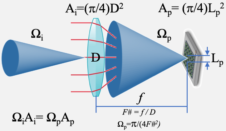
Simple optical system conversions	In an idealized optical sytem, the incidence etendue is equal to the sampled etendue by the detector. The tool below allows to perform simple conversions applying this principle:   Ai [m2] Di [m] Ωi [sr] Θi [rad] Θi [arcsec] Ap [m2] Lp [m] Ωp [sr] F-number [f/F#]     Inputs Ai [m2] Di [m]   Ωi [sr] Θi [rad] Θi [arcsec]   Ap [m2] Lp [m]   Ωp [sr] Θp [rad] Θp [arcsec] F-number [f/F#]

 
The noise components with Poisson statistics (i.e., UV, optical, IR) are calculated as:
 
L_e- = Ω ⋅ A_Tele ⋅ η_eff ⋅ dλ ⋅ λ ⋅ t_exp ⋅ n_exp ⋅ 1E-6 / hc        Radiance to detector electrons conversion factor
 
N_source = L ⋅ L_e-        Noise introduced by the source itself [e-²]
 
N_back = (L_back + n_ezo⋅L_zodi) ⋅ L_e-        Noise introduced by background sky sources [e-²]
 
N_optics = ε_optics ⋅ L_e- ⋅ (2E24 ⋅ h ⋅ c² / λ⁵) / (exp(1E6 ⋅ h ⋅ c / (k ⋅ T_optics ⋅ λ)) - 1)        Noise introduced by the telescope [e-²]
 
N_ground = L_e- ⋅ (1 - trn_ground) ⋅ (2E24 ⋅ h ⋅ c² / λ⁵) / (exp(1E6 ⋅ h ⋅ c / (k ⋅ T_ground ⋅ λ)) - 1)    Noise for ground observations [e-²]
 
N_Total = √(2N_D + N_source + 2N_back + 2N_optics + 2N_ground)        Total noise [e-]
 
Assuming these parameters and units:
    L [W / sr / m² / μm]: spectral radiance of the source
    L_back [W / sr / m² / μm]: spectral radiance of the background sources
    t_exp [s]: time per exposure
    n_exp: total number of exposures
    n_pixels: total number of pixels for Ω and dλ.
    n_ezo: Exozodiacal dust scaler relative to Solar System zodiacal dust
    T_optics [K]: temperature of the optics
    ε_optics: emissivity of the optics
    η_eff: total throughput of the system (including quantum efficiencies)
    Ω [steradian]: is the solid angle of the observations. It is wavelength dependent.
    A_Tele [m²]: is the total collecting area of the observatory (n_Tele⋅π⋅[D_Tele/2]²)
    λ [μm]: is the wavelength in microns
    trn_ground: terrestrial transmittance
    T_ground [K]: temperature of the terrestrial atmosphere - 280
    h [W s²]: is Planck's constant - 6.6260693E-34
    c [m / s]: is the speed of light - 299792458
    k [J / K]: is Boltzmann's constant - 1.380658E-23
 

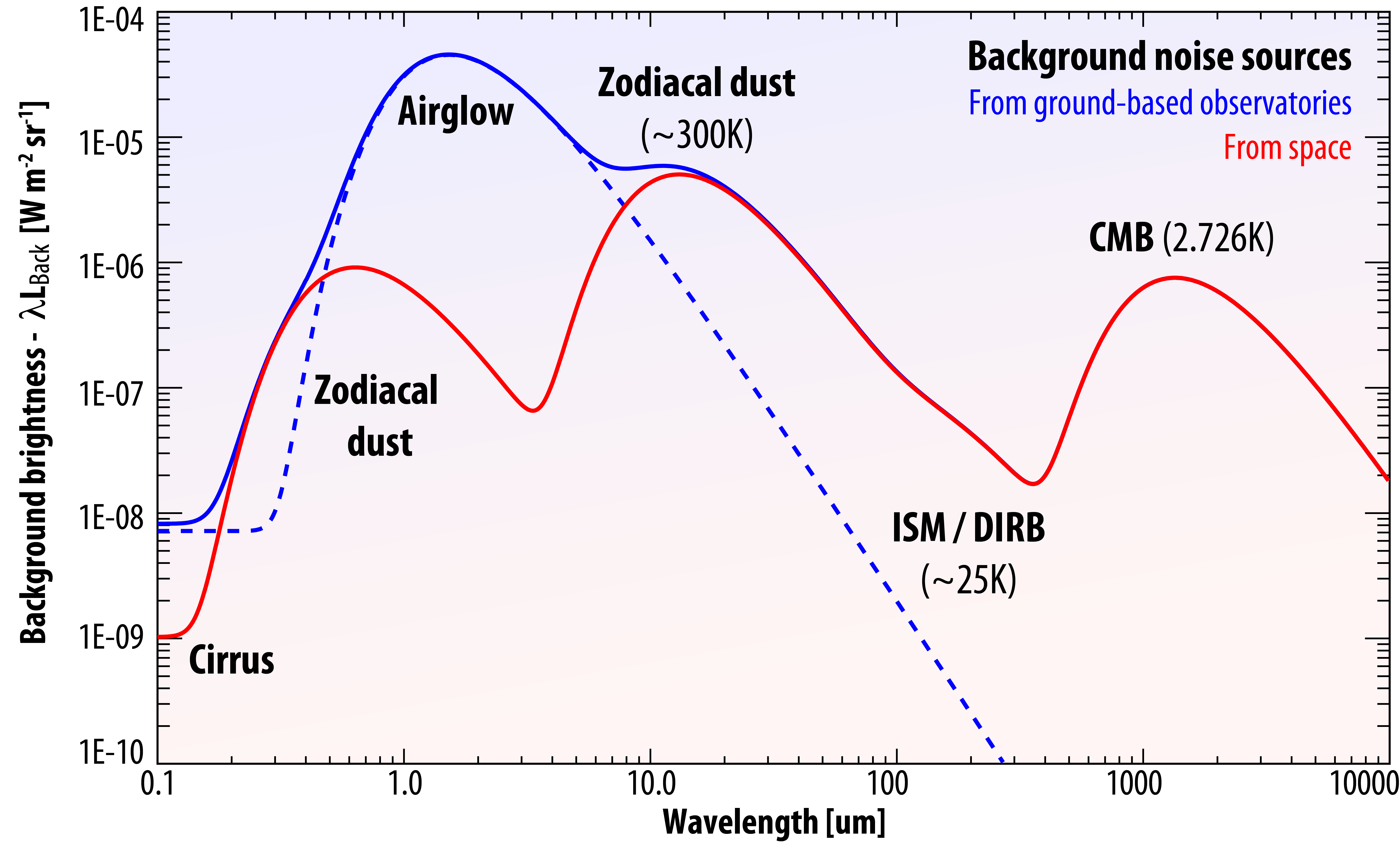Background noise sources: When observing faint astronomical sources, the sensitivity is affected by the shot noise introduced by background and diffuse sources (Leiner et al. 1998, A&A, v.127, p.1-99). From space, the background is dominated by the faint and diffuse emission (thermal and scattered sunlight) from zodiacal dust, while airglow (a mixture of photoionization emissions, chemiluminescence and scattered sunlight) dominates the background for ground-based observations. PSG also employs a rudimentary (as shown), yet relatively effective, approximation for atmospheric airglow. Details about the scaling of the zodiacal background fluxes is explained below.

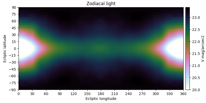
Zodiacal levels

The zodiacal light is the faint and diffuse radiation across the ecliptic plane originating from scattered sunlight by interplanetary dust. The brightness of the zodiacal light decreases with distance from the Sun, with a notable increase at opposition due to backscattered sunlight ("gegenschein"). This background radiation is typically the main background radiation term impacting space observations of faint objects, and it is highly dependent on the RA/DEC of the target and the time of the observations.
 
In PSG, the parameterization of the zodiacal level is done by a scaling factor with respect to the polar ecliptic value (23.3 V mag/arcsec²), with a scaling of 2 (22.5 mag/arcsec²) being the default and the typical value for a general observatory. For exozodis, the surface brightness increases because of the geometry and preferable scattering with an average value of 22 V mag/arcsec². In coronagraphy, the user can scale this by a multiplier (1 being 22 mag/arcsec²]).
 

The zodiacal flux decreases notably when away from the Sun, and as the Sun moves across the sky (RA/DEC) during the year, the zodiacal levels change for the same RA/DEC. It is therefore of importance to properly define the zodiacal level at the time of the observations or at the most favorable time/month. The calculator below permits to estimate the zodiacal level and the scaler to be used in PSG. The levels shown in these figures were computed by combining data from Kwon et al. 2004 and from Leiner et al. 1998. The table is accessible here.
Coordinates RA/DEC Ecliptic Galactic Time/month Best moment January February March April May June July August September October November December