Planetary

Types of atmospheres

PSG handles two types of atmospheres: hydrostatic equilibrium (typical for planets) and expanding coma (i.e., exospheres and typical of comets and small bodies). Atmospheres in hydrostatic equilibrium are considered when gravity controls the structure of the atmosphere and in which the escape velocities are lower than the kinetic atmospheric velocities. For exospheres, the structure is defined by the outgassing velocity and photochemical/photodissociation decay, while in hydrostatic equilibrium, gravity, molar mass, pressures and temperature define the vertical structure. PSG permits providing detailed vertical information of molecular abundances and temperatures, and atmospheric templates (vertical profiles of temperature and abundances) are available for the main atmospheres (Venus, Earth, Mars, Titan, Neptune, Uranus), while general atmospheric and surface parameters are available for the other bodies. For expanding atmospheres, PSG assumes isotropic outflow, constant expanding velocity and a Haser isotropic 2-steps (i.e., parent and daughter species) photodissociation scheme.
 
PSG provides access to several atmospheric models (e.g., chemical equilibrium, thermal radiative equilibrium, Mars GCM models, cometary heliocentric models), databases (e.g., Earth NASA/MERRA2) and numerous templates (e.g., Venus, Titan) for defining the atmospheric and surface structure and composition. The user can also provide any arbitrary profile of P/T and of molecular abundances by selecting "File Template" in the atmosphere section. The format of this file is a text file with all the entries as in the configuration file for the sections ATMOSPHERE and SURFACE. When providing user-generated profiles, the vertical parameters are provided via the ATMOSPHERE-LAYER keywords. The pressures are provided in 'bars', temperatures in 'K' and abundances in volume mixing ratio - [molecules / molecules] for gases (e.g., water vapor, methane) and [kg / kg] for hazes (e.g., water ice clouds, methane ice). Particle sizes in [m] are provided by adding the keyword '_size'. The base (molecules or kg) is always wet air (all gases, including water vapor) without hazes. When no vertical profile is provided, the temperature (T) is assumed to be constant across the atmosphere, and the pressure (P) decreases with altitude (z) following the scale-height: P = Psurf exp(-zg/RT), where g is the gravity (defined in the object section) and R is the gas constant (8.3144598 J / K / mol).
 
It is important to note that only molecules included in the ATMOSPHERE-GAS and ATMOSPHERE-AEROS will be included in the simulation, independent of the species included in the profiles. Specifically, the vertical profile/structure of the atmosphere is provided by the ATMOSPHERE-LAYER keywords, yet the connection between these profiles to the species listed in the ATMOSPHERE-GAS field is done via the “scaler” abundance unit in the ATMOSPHERE-UNIT keyword (see details in chapter 1 and explore an example config in PSG for further understand this connection). A scaler of 1 indicates that the values as in the profile will be used, while any other unit (e.g., ppm, ppb) indicates a constant mixing ratio with altitude. If a scaler is selected for a constituent for which no profile exists, PSG will consider a scaler relative to an abundance of 100%. The surface pressure indicates where the atmosphere starts, again independently of the profile pressures. The surface pressure is where the surface starts, and where the diameter and gravity values relate to in the vertical structure of the planet.
 

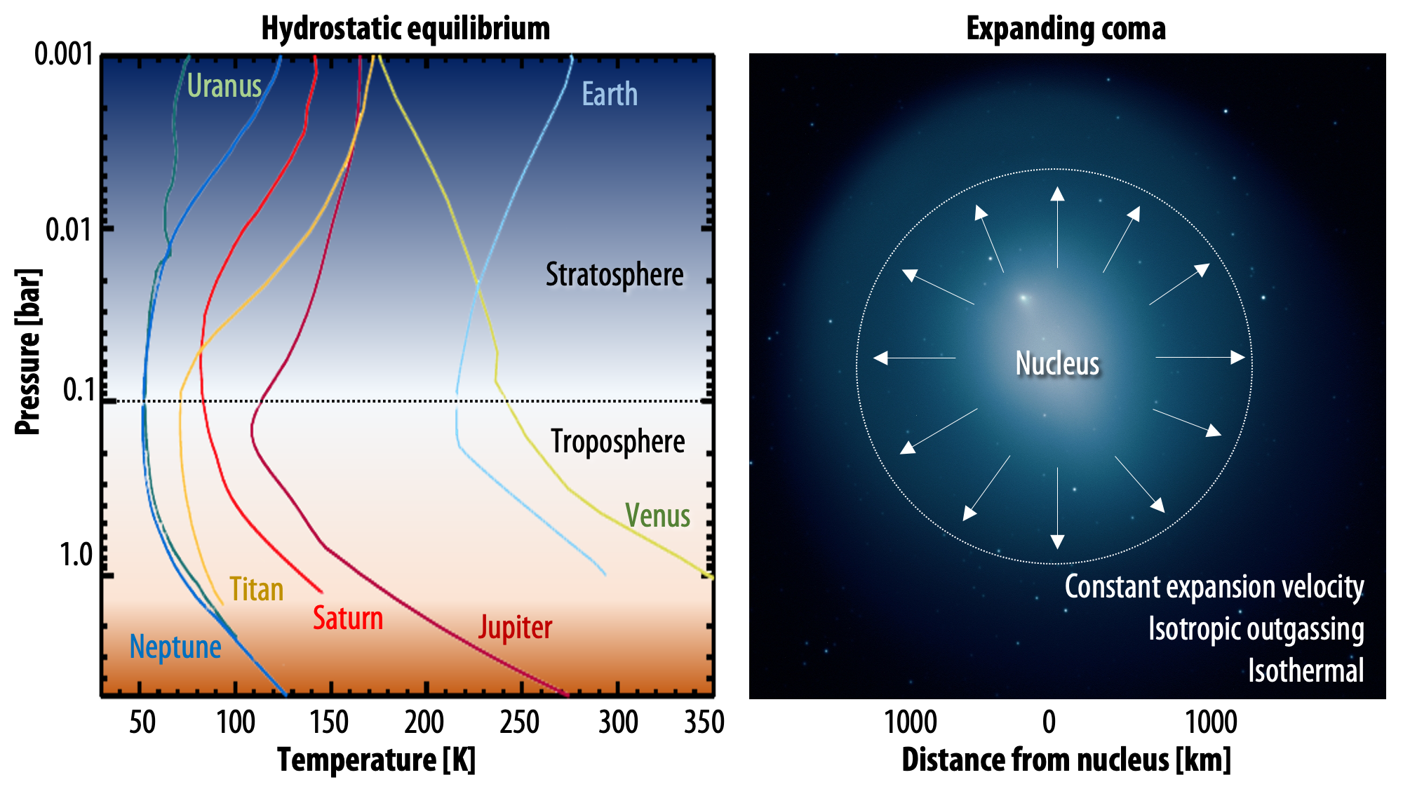Types of atmospheres: the user can select between two types of atmospheres: hydrostatic equilibrium (typical for planets, profiles adapted from Robinson & Catling 2014) and expanding coma (typical of comets and small bodies). For the main planets, vertical profiles are available, while the user can also load any arbitrary vertical structure. For expanding atmospheres, PSG assumes isotropic outgassing, a constant temperature across the coma, and an outgassing velocity established by the heliocentric distance.

When selecting the spectroscopic databases for each of the atmosphere, aerosols and surface components, the user can choose from the following types:
 

 
 

Molecular/atomic databases (8680 species)

Download full list

The key parameter to be entered in the "Atmosphere" section is the definition of the molecular species and the corresponding linelist to be used for these molecules. HITRAN is generally very complete (for IR, optical and UV at low temperatures) for most typical planetary atmosphere and has become the main repository of line information. At radio wavelengths, the JPL Molecular Spectroscopy and Cologne Database of Molecular Spectroscopy (CDMS) are generally more complete and have a better description of the rotational spectrum of complex molecules. NASA-Goddard currently holds the main repository for non-LTE fluorescence linelists, suitable when synthesizing cometary spectra in the UV/optical/IR range.
 

Database	Capabilities	Reference
HITRAN/HITEMP 2020	Wavelength range: 0.3 μm to radio Number of lines: 5,399,562 Number of molecules: 50 Number of isotopologues: 126 Number of cross-section spectra: 987 Number of aerosols: 98	Gordon, I.E. et al; "The HITRAN2020 molecular spectroscopic database", Journal of Quantitative Spectroscopy and Radiative Transfer 277, 107949 (2022)
	Correlated-k tables Wavelength range: 0.2 to 100,000 um Number of temperatures: 20 (40 to 2000 K) Number of pressures: 17 (1E-6 to 100 bar) Number of species: 21	Absorption coefficients computed with PUMAS, and assuming wings of 25 cm-1 and a fine core of 1 cm-1 where maximum resolution calculations are applied. Molecules: H2O, CO2, O3, N2O, CO, CH4, O2, SO2, NO2, NH3, HCl, OCS, H2CO, N2, HCN, C2H2, C2H4, PH3, H2S, C2H4, H2
	HOT correlated-k tables Computed based on the H2O, CO2, CO and CH4 HITEMP databases, assuming average line parameters in different collisional regimes (e.g., air, CO2, H2, He), and only available for low-res simulations (RP≤500).	Rothman, L. S. et al., "HITEMP, the high-temperature molecular spectroscopic database", JQSRT 111, 2139-2150 (2010) - With updates up to Feb/2023
GSFC Fluorescence Database      Download	Wavelength range: shorter than 10 μm Number of lines: 530,281 Based on lines (non-LTE): 2 billions Number of species: 26 For daughter species, rotational populations are heavily affected by photodissociation, and for simplicity in PSG, we assume an elevated Trot of 600K for OH,CN,CH,NH and 3200K for C2.	Villanueva, G. L., Mumma, M. J., DiSanti, M. A., Bonev, B. P., Gibb, E. L., Magee-Sauer, K., Blake, G. A., Salyk, C., "The molecular composition of Comet C/2007 W1 (Boattini): Evidence of a peculiar outgassing and a rich chemistry". Icarus, Volume 216, Issue 1, p. 227-240. (2011)
	For rotational transitions, full non-LTE calculations are computed by solving the multi-level system of differential equations in an expanding coma considering a time-dependent solution. Collisional parameters with H2 (assuming thermal OPR) are compiled following the LAMDA database (Leiden Atomic and Molecular Database, Schoier et al. 2005). Spectroscopic line information is compiled from various sources (ExoMol, HITRAN2020, LAMDA as presented in Villanueva et al. 2012a/2012b/2013), with fluorescence pumping rates (G coefficients) computed based on multi-cascade analysis considering billions of transitions. The pumping rates were computed considering a realistic solar spectrum at Rh=1AU and a heliocentric velocity of +10 km/s. See below the non-LTE model and the compiled databases: Model C2 CH CH3OH CN CO CO_1217 CO_1218 CO_1316 H2CO H2O H2S  HC3N HCN HDO HNC NH NH3 OCS OH
GEISA 2020	Wavelength range: 0.3 μm to radio Number of lines: 5,023,277 Number of species: 52 Number of isotopologues: 118	Jacquinet-Husson, N. et al; "The 2020 edition of the GEISA spectroscopic database"; Journal of Molecular Spectroscopy, Volume 327, Pages 31-72 (2016)
JPL Molecular Spectroscopy	Wavelength range: 2.65 μm to radio Number of lines: 888,113 Number of species: 383	Pickett, H. M.; R. L. Poynter, E. A. Cohen, M. L. Delitsky, J. C. Pearson, and H. S. P. Muller, "Submillimeter, Millimeter, and Microwave Spectral Line Catalog"; J. Quant. Spectrosc. and Rad. Transfer 60, 883-890 (1998)
CDMS Cologne Database for Molecular Spectroscopy	Wavelength range: 1.81 μm to radio Number of lines: 1,612,154 Number of species: 792	Muller, Holger S. P.; Schloder, Frank; Stutzki, Jurgen; Winnewisser, Gisbert; "The Cologne Database for Molecular Spectroscopy, CDMS: a useful tool for astronomers and spectroscopists"; Journal of Molecular Structure, Volume 742, Issue 1-3, p. 215-227 (2005)
EXO-Transmit database      Download	Wavelength range: 0.1 to 170 um Number of spectral points: 7454 Number of temperatures: 30 (100 to 3000 K) Number of pressures: 13 (1E-9 to 1000 bar) Number of species: 30	Freedman et al. 2008, 2014, from ExoTransmit - Kempton+2017, PASP 129-044402, https://iopscience.iop.org/article/10.1088/1538-3873/aa61ef/meta, Exo-Transmit
The MPI-Mainz UV/VIS Spectral Atlas	Wavelength range: 0.01 to 1 um Number of cross-sections: 52 (selection) Number of species: 22 (selection)	Keller-Rudek, H., Moortgat G.K., Sander R., Sörensen R., "The MPI-Mainz UV/VIS Spectral Atlas of Gaseous Molecules of Atmospheric Interest", Earth Syst. Sci. Data, 5, 365–373 (2013) Venot et al., A&A, 609-A34 (2018) Serdyuchenko et al.,Atmos. Meas. Tech., 7, 625-636, 2014
The CFA/Harvard Kurucz atomic database	Wavelength range: 0.001 to 1000 um Number of species: 80 elements and their ions Number of lines: 2,309,497	Kurucz, Smith, Heise, Esmon (gfall08oct17), "The CFA/Harvard Kurucz Atomic spectral line database" (2017)'
	Modeling: the model of the lineshapes includes a Voigt analysis (Thermal, Natural, van-der-Waals) within the impact theory region and an extended wing region beyond for the statistical regime. The transition between these regimes is defined by the detuning frequency (Nefedov+1999, Burrows+2000, Iro+2005). Einstein Aul [s-1] = gf / (1.499E-14 ⋅ (2J+1) ⋅ λ2)   where gf is the tabulated oscillator strength, J is the upper-state rotational number and λ is the wavelength [nm]. Natural halfwidth [cm-1] = γrad / (4πc)   where γrad [s-1] is the radiative damping constant and c the speed of light [cm/s]. Collissional halfwidth [cm-1/atm] (T/296)-0.7 = γ6 ⋅ 8.62489e+18 / (4πc)   where γ6 [s-1] is the van der Waals damping constant (neutral hyrogen) and T is the temperature [K]. Detuning frequency [cm-1] = 25 ⋅ [T/(ma⋅250)]0.5   in this approximation, ma is the molar mass [amu] of the atmosphere. Extended lineshape model = (v-v0)-3/2⋅exp(-h(v-v0)/kT)   where v0 is the line center [cm-1].
Continuum processes	Rayleigh molecular scattering: Rayleigh scattering results from the electric polarizability of the molecules/atoms. The oscillating electric field of a light wave acts on the charges within a molecule/atom, causing them to move at the same frequency. The molecule/atom, therefore, becomes a small radiating dipole whose radiation we see as scattered light. The treatment of Rayleigh in PSG follows the methodology described in Sneep & Ubachs (2005, JQSRT), in which each molecule/atom is added following their polarizability Table   Raman molecular scattering: At wavelengths approaching the size of the molecules, the oscillating electric field of a light wave acts on the charges within a particle, leading to the molecule to become a radiating dipole. Rayleigh results from the elastic scattering of radiation, while a small fraction is scattered inelastically, with the scattered photons having an energy different (usually lower) from those of the incident photons - these are Raman scattered photons. In PSG, we model Raman following the original method developed by (Pollack et al., 1986), which has been adapted to include the Raman cross sections for H2 and N2 computed by (Oklopčić et al., 2017).   Refraction: refraction is the change in direction of light as it progresses along the atmosphere with gradually changing refraction index. How much the light is refracted is determined by the change in wave speed and the initial direction of wave propagation relative to the direction of change in speed, and can be modelled following Snell’s law. PSG considers four possible scenarios for refraction a) H2 atmosphere for molar masses lower than 3 g; b) He atmosphere for molar masses 3 to 10; c) air [N2/O2] atmosphere for molar masses 10 to 35; and d) CO2 atmosphere for molar masses greater than 35. The refraction indexes constants are compliled from refractiveindex.info.   Collission-induced absorption (CIA): collision-induced absorption and emission are generated by inelastic collisions of molecules in a gas. Such inelastic collisions (along with the absorption or emission of photons) may induce quantum transitions in the molecules, or the molecules may form transient supramolecular complexes with spectral features different from the underlying molecules. Collision-induced absorption and emission is particularly important in dense gases, such as hydrogen and helium clouds found in astronomical systems. The available CIAs datasets (from HITRAN and references therein are): CH4-Ar CH4-CH4 CH4-He CO2-Ar CO2-CH4 CO2-CO2 CO2-H2 CO2-He CO2-O2 H2-CH4 H2-H  H2-H2 H2-He H2O-H2O H2O-N2 He-H N2-CH4 N2-H2 N2-H2O N2-He N2-N2 O2-CO2  O2-N2 O2-O2  PSG integrates the MT_CKD water continuum (v3.5, Payne et al. 2021) by transforming it to CIAs (Kofman & Villanueva 2021):  Self  Foreign   Ultraviolet (UV) broad absorptions (λ < 1.0 μm): The high energies (optical/UV/EUV) of a molecule are normally described by a non-quantizied broad swath of energy levels. Many of these highly energetic levels lead to the photodissociation/disintegration of the molecule. The spectroscopic signatures for a molecule in this domain are typically not captured by classical linelists, and therefore PSG complements linelists by including cross-sections from the MPI-Mainz UV/VIS Spectral Atlas and other UV databases/references.

 

Search  Molecule  Type
	Download Partition functions Vibrational levels

 

Opacity generator

Search  Molecule  Type
Frequency/wavelength range: um nm mm Angstrom cm-1 MHz GHz kHz    Resolution: Resolving power um nm mm Angstrom cm-1 MHz GHz kHz
Pressure: bar Pascal kbar mbar ubar at atm Torr psi Temperature [K]:   Threshold (for linelist):	%     %     %     %     %	The collissional and excitation environment will be based on these parameters and the availability of spectroscopic information (see databases above).
Generate linelist Generate opacities

 

Scattering aerosols (101 species)

Download full list

As light travels across an atmosphere, it is absorbed (then transformed into heat and thermally emitted) and it is also scattered into many directions. Scattering in this sense, refers to the reflection and deflection of photons in a 3D manner across an atmosphere. When this process is active in an atmosphere, it leads to an “ambient” diffuse shine and a peculiar light pattern when looking close to the Sun. For instance, when no scattering is active (only absorption), we would have black skies with only a point source of light at the location of the Sun. Molecular Rayleigh scattering is the reason we have blue skies, in which molecules “scatter” in many directions, and in which photons are scattered towards the observer even when the Sun is quite far from the observed patch of the sky. As can be quickly inferred, computing scattering is therefore a 3D problem, which can be numerically extremely difficult to solve since photons need to be tracked across the full three-dimensions (azimuth angle, polar angle, depth/altitude). In a non-scattering medium, the solution of the radiative transfer equation is straightforward, with only needing to track the photons as they go through the incidence and emission paths. For such case, PSG can solve this integro-differential equation readily and efficiently without needing to solve any multiple scattering 3D problem.
 
Ultimately, solving a full 3D integro-differential scattering problem for the myriad of possible incidence and emission angles would appear in principle unattainable. Several methods do exist, and these include the doubling-adding method, the discrete ordinates approach, the successive orders of scattering method, Gauss-Seidel iteration, and the Monte Carlo approach, among others. In particular, Chandrasekhar introduced in 1940 a pioneering method for solving radiative transfer in a scattering medium, the discrete ordinate method. The primary merit of this method is that it reduces the integro-differential equation to a system of ordinary differential equations, and it divides the scattering directions into numerical series. The foundation math and the proposed numerical implementation are still at the core of the most popular modern scattering methods, yet the original implementation suffered from many numerical and stability issues, and basically doomed Chandrasekhar’s analytic approach for any but the isotropic and Rayleigh scattering problems. In the 1970s, the discrete ordinate method was further improved and many numerical enhancements were developed to improve its accuracy (e.g., Liou, 1973; Wiscombe, 1977). These codes were still plagued with instabilities and issues at high opacities, requiring exorbitant number of computational layers and scattering polar angles. For instance, in the popular delta-Eddington method, the high opacity instability was sidestepped by subdividing layers until each sub-layer was optically thin, which was extremely computational expensive or impractical for many problems.
 
In the 1980s, the foundational work by Stamnes and others, led to the now widely used DISORT package (Stamnes et al., 2000, 1988), which captures the pioneering discrete ordinate math by Chandrasekhar, the improvements done in the 1970s and finally solved the many issues affecting this method (e.g., stable for high opacities, accurate for low number of polar angles). Since its inception, DISORT has been constantly updated and improved, yet the core foundational concepts have not substantially changed since then. In PSG, we employ the core methods of DISORT 2.1 written in C by Dowling and colleagues (Buras et al., 2011) which we adapted for non-LTE and optimized to operate with a variety of spectral grids (e.g., line-by-line, correlated-k, surface scattering grids) as employed by the PSG radiative transfer algorithm. The model includes correction for pseudo-spherical geometry as described by (Dahlback and Stamnes, 1991).
 

Molecular (Rayleigh) and aerosols (Mie) scattering

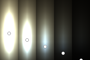
The two main processes dominating scattering in an atmosphere can be separared into molecular (Rayleigh) scattering and aerosols (Mie) scattering. Molecular scattering results from the electric polarizability by molecules, which are much much smaller than the wavelength of the radiation. The amount of scattering is inversely proportional to the fourth power of the wavelength, so its effects is prominently at short wavelengths (lower than 1 micron). Aerosols scattering can be modelled employing Mie theory (Rayleigh scattering can be also described with Mie theory), and therefore this type of scattering by small particles is called Mie scattering. Molecular scattering tends to be more isotropic, while aerosols scattering is more promiment at wavelengths comparable to the size of the particles, and tends to have a very directed phase function, leading to notable asymmetries in the observed fluxes with respect to phase angle. In the examples below, we show synthetic all-sky images computed with PSG considering molecular scattering and aerosols scattering for several planets (e.g., Earth, Mars, Titan, Uranus) and aerosol content.
 

Earth	Cloudy Earth	Overcast Earth
Dusty Mars	Hazy Titan	Uranus
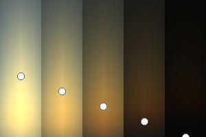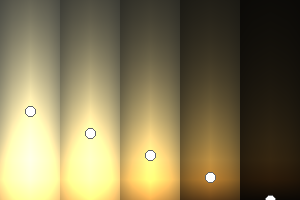
Atmospheric scattering: As the Sun moves across a planetary atmosphere, its photons are scattered in different directions with a pattern defined by the wavelength of the photons. The slices top/bottom panels show the sunset for zenith angles (70,75,80,85,90) at a solar azimuth angle of +/-20 and for observational zenith angles below 45 degrees. The middle animations show all-sky views for different solar zenith angles. As it is shown for Earth’s clear atmosphere, the scattering pattern is mostly symmetric when Rayleigh dominates, while when clouds are added a non-symmetric halo is added towards the Sun direction because of Mie aerosols scattering. In the case of Mars, the atmosphere switches from a ‘brownish’ color to a ‘blueish’ tint at high solar zenith angles due to the preferential Mie scatter of Mars dust particles at red wavelengths.

 
Converting aerosol abundances: PSG ingests aerosol abundances f in [kg/kg] or [g/g], yet many references report aerosols in several different units. If one uses the scattering models computed in PSG, these incorporate a log-normal distribution with S=1.5, then exp(-3ln²S) = 0.6107 (more information in chapter 5 of the handbook). A common unit is N [particles/cm3], to determine X [kg/kg] for N=1 [particles/cm³], P=5e-3 [bar], T=340 [K], m_atm=18 [g/mol], particle radius (not diameter) r_haze=1e-5 [cm], ρ_haze=1.36 [g/cm³], N_A [6.022140857e23 molecule/mol]:
 
V_haze = π (4/3) ⋅ r_haze³ = 4.2e-15 [cm³] Volume of each haze particle
m_haze = V_haze ⋅ ρ_haze ⋅ exp(-3ln²S)= 3.5e-15 [g]
ρ_atm = 1E-1 ⋅ P / (KB [1.38064852e-23] ⋅ T) = 1.065e+17 [molecules/cm³]
f_haze = N ⋅ m_haze ⋅ N_A / (ρ_atm ⋅ m_atm) = 1.1E-9 [g/g] (aerosol mass abundance)
 

 

Search  Aerosol
	Download

Defining the surface

As light arrives to a surface at a particular wavelength, it can be either be absorbed or scattered. Processes such as surface fluorescence or Raman will transfer some of this energy to a different wavelength, but for our treatment in PSG, we simply consider this as an absorption process at this wavelength. The direction and intensity of the scattered light requires of complex modeling, and several methods exist (e.g., Lambert, Hapke). The light absorbed will heat the surface, and this together with other internal sources of heat will lead to thermal emission (with an associated directionality and effectiveness/emissivity). How effective the surface scatters light is defined by the single scattering albedo, where 0 means the light is totally absorbed and to 1 the light is totally scattered back.
 
What is being observed or “reflected” back will depend on how this surface scatters back, and we would then require information about the observing geometry, the directability of the emissions and the geometry of the incidence fluxes. Three angles are used to define the geometry: i “incidence angle” is the angle between the Sun (or host-star) and the line perpendicular to the surface at the point of incidence, called the normal; e “emission angle” is the angle between the surface normal and the observer; and g “phase angle”, which is the angle between the source and observer (not to be confused with solar azimuth angle, which is the projection of the phase angle).
 
The quantity that captures how much light is being reflected towards the observer is called r(i,e,g) “bidirectional reflectance”, which is in units of per [sr], with steradians [sr] being a unit of solid angle. A common alternative quantity is the BRDF or “bidirectional-reflectance distribution function”, which describes the reflectivity of the surface with respect to a Lambertian sphere, and it is simply r/cos(i). Similarly for emission, directional emissivity is the ratio of the thermal radiance emerging at emission angle e from the surface with temperature T with respect to a black body at the same temperature.
 
Once the geometry (i,e,g) and the specific scattering properties (e.g., ) are defined, we would then need a scattering model to accurately model the emissions from a sphere. In PSG, four core models are available: Lambert (isotropic scattering), Hapke (parametric surface scattering), Lommel-Seeliger (weakly scattering / diffuse surfaces) and Cox-Munk (specular glint scattering model).
 
 

Surface materials (29568 components)

Download full list

Properly modeling spectroscopic features of planetary surfaces over a wide wavelength range requires a comprehensive and inclusive spectroscopic database. These parameters are used to establish the "boundary" conditions for the radiative transfer calculations. There is currently no single repository that integrates optical constants and reflectances of solid surfaces and ices over a wide spectral range (only specialized databases exist). We have identified eleven spectral databases that are applicable to the synthesis of planetary spectra, and we have developed a program to standardize and homogenize these libraries of spectral constants.

• RELAB Reflectance Experiment Laboratory
• NASA Goddard's Cosmic Ice Laboratory
• NASA Ames' Database of Astrochemical Ices
• NASA ASTER Spectral Library
• The PDS Geosciences Spectral Library
• MRO CRISM Type Spectra Library
• USGS Digital Spectral Library
• Grundy's optical constants of Ices
• PDS Ices database
• Database of Optical Constants for Cosmic Dust
• Grenoble Astrophysics and Planetology Solid Spectroscopy and Thermodynamics database service

 

Search  Component
	Download